Ciencia, Ingenierías y Aplicaciones, Vol. 7, No. 1, enero-junio, 2024 ISSN (impreso): 2636-218X • ISSN (en línea): 2636-2171
ESTIMATION OF SPECIFIC TRACTION ELECTRIC POWER CONSUMPTION FOR BOGOTÁ METRO FIRST LINE
Estimación de consumos específicos de energía eléctrica de tracción para la primera línea del Metro de Bogotá
DOI: https://doi.org/10.22206/cyap.2024.v7i1.3102
LUIS HERNANDO CORREA SALAZAR1
Recibido: 25/03/24 • Aceptado: 29/04/24

Cómo citar: Correa Salazar, L. H. (2024). Estimation of specific traction electric power consumption for Bogotá Metro First Line. Ciencia, Ingenierías y Aplicaciones, 7(1), 5–31. https://doi.org/10.22206/cyap.2024.v7i1.3102https://doi.org/10.22206/cyap.2024.v7i1.3102
Abstract
This study aims to identify the mechanical variables that exert the greatest influence on the consumption of traction energy in a metro-type system, estimate specific energy consumption in different operating scenarios associated with speed profiles in each section and establish specific reference consumptions that guide the identification of projects aimed at increasing energy efficiency, all estimated for when the first line of the Bogota Metro comes into operation. To achieve the previous objectives, this research was focused on the estimation, through a software application, of the specific consumption of electrical energy of the Metro System of the City of Bogota, for different operating scenarios. Results of simulations carried out with an application developed in Matlab, to generate speed profiles in the operation of the train, allow observing the sensitivity of the specific consumption of electrical energy in the face of changes made in the cruise speed and in the acceleration ramps and slowdown. The results show that the specific consumptions depends to a great extent, on the speed profiles, and consequently on the operation of the system, which opens an interesting field of application of optimization techniques oriented to the efficient use of energy in the future operation of the system.
Keywords: Electric power; energy consumption; train; urban traffic; expenditure.
Resumen
Este estudio tuvo como objetivos identificar las variables mecánicas que ejercen mayor influencia en el consumo de energía de tracción en un sistema tipo metro; estimar el consumo específico de energía en diferentes escenarios operativos asociados a perfiles de velocidad en cada tramo y establecer consumos de referencia específicos que guíen la identificación de proyectos orientados a incrementar la eficiencia energética cuando entre en operación la primera línea del Metro de Bogotá. Para lograr los propósitos anteriores, esta investigación se centró en la estimación, a través de una aplicación de software, del consumo específico de energía eléctrica del Metro de la Ciudad de Bogotá, en diferentes escenarios operativos. Resultados de simulaciones realizadas con una aplicación desarrollada en Matlab, para generar perfiles de velocidad en la operación del tren, permiten observar la sensibilidad del consumo específico de energía eléctrica ante cambios realizados en la velocidad de crucero y en las rampas de aceleración y desaceleración. Los resultados muestran que los consumos específicos dependen, en gran medida, de los perfiles de velocidad y del funcionamiento del metro, lo que abre un interesante campo de aplicación de técnicas de optimización orientadas al uso eficiente de la energía en la futura operación del sistema.
Palabras clave: Energía eléctrica; consumo de energía; tren; tráfico urbano; costo.
1. Introduction
Massive transport systems represent a great load for the distribution circuits of cities and are large consumers of electrical energy, constituting, therefore, important systems when identifying potential opportunities for savings and improvement in the efficient use of energy. A key indicator in energy efficiency is the so-called specific energy consumption (energy per unit of production), which can be established as a reference point in the monitoring of projects associated with the increase in efficiency and productivity and which also finds application in studies and analysis of comparison of energy consumption per unit of production between different companies, entities, systems and modes of transport, etc. The specific consumption indicator is well known by energy managers and is very often used in companies of an industrial manufacturing nature and also of continuous flow, but it is little used in other activities such as mass transportation systems that use electrical energy as an input. Difficulties of various kinds such as lack of information regarding the “unit of production” of these systems and the difficulty in identifying the variables that exert a greater influence on energy consumption hinder their use, thus causing a problem that prevents, among other things, having reliable reference and comparison points for the adequate integral management of energy.
This research is focused on the estimation, through a software application, of the specific consumption of electrical energy of the Metro System of the City of Bogota, in different operating scenarios. The central focus of interest is the energy consumed by the traction subsystem (subsystem responsible for the movement of the train), which represents between 40 percent and 80 percent of the total energy consumed by these massive transport systems. The approach in the estimation of specific energy consumption is made taking into account key mechanical variables in the operation, such as acceleration and deceleration rates and steady-state or cruising speed in each of the sections that constitute the first line of the Bogota Metro. A crucial aspect that has emerged in recent years, and due to pressures from environmental groups, has to do with the introduction of technological innovations that tend to reduce energy by using regenerative braking in deceleration; it is worth mentioning that potentials of up to 50 percent of the energy generated in braking could be returned to the electrical power distribution system.
In calculating the energy needed by a metro-type system, the determination of the traction force to produce the movement is key, which is a function of mechanical variables such as the weight of the train, the number of passengers, the average weight of the passengers and the instantaneous speed. In the international arena, and for several decades, enough experience and knowledge has been gained to determine the traction force needed in railway systems, so much so that there is a reliable equation (modified Davis equation) for the calculation of the instantaneous traction force. Once you have the instantaneous force, the next step is the calculation of the instantaneous power and then its integration over time to quantify the total energy for an entire path of a certain length. Knowing the total energy and length, can be determined the indicator of specific energy consumption, which has units of electrical energy per unit length for each train, this is different according to the number of users that are transported.
A first work that can be mentioned, related to energy efficiency in massive metro-type transport systems, addresses the reduction of energy consumption from the point of view of the system as a whole and considers measures aimed at improving the operation and implementing technology (González et al, 2014). The paper concludes that there are several measures that have proven to be successful and that a key aspect in the implementation of these measures is the continuous monitoring of representative indicators that are identified.
The research work of Gao et al. (2018), focuses on an analysis of energy consumption and time spent on the route between stations of metro-type systems, considering two modes of operation. The work identifies interesting potential for energy savings by introducing improvements in the operation of the routes; however, it does not focus on monitoring indicators for the purpose of observing improvements (decreases in energy consumption) in savings achieved.
The work of Gatusso & Restuccia (2014), examines various cost estimation methodologies and develops cost functions involving specific energy consumptions for regional rail transport systems with different fuels (diesel, gas, electricity). The work presents a specific reference consumption for regional trains, varying between 3.5 and 5.5 kWh/(km.train) at European level; Unfortunately, the focus of the study is on regional trains and not massive Metro-type transportation systems. In the work of Domínguez et al. (2012), the fundamental interest is the reduction of energy consumption through the use of automatic operating systems, which select, online, speed profiles within a pre-established set of optimized profiles. In the work they propose the design of an automatic operation system with pre-established profiles taking into account the energy recovered with regenerative braking to reduce the consumption of energy extracted from the substations that feed the Metro system. The work is based on a case study on line 3 of the Madrid Metro (17 stations, with a total of 13.5 km per direction), a line in which they obtain, through numerical simulation, average values of energy consumed in traction and energy recovered with regenerative braking. Average values of 12.91 kWh /(km.train) are reached for the specific traction energy and 3.69 kWh/(km.train) for the specific energy returned to the grid by regenerative braking. With the above values, and with several defined scenarios, optimized profiles are proposed and energy savings are estimated.
Two points can be stressed about the existing work. On the one hand, that energy can be managed to make efficient use of it. On the other hand, the aforementioned studies also establish the recommendation to identify key indicators for monitoring and follow-up in energy reduction projects. As key indicators, cost functions and specific consumption indicators are available, since they constitute tools for planning and making public policy decisions.
The contribution of this work consists of determining specific consumption of electric traction energy, in different operating scenarios of the first line of the Bogota metro. These specific consumptions constitute reference points for undertaking actions aimed at improving the energy efficiency of a large energy-consuming system such as a metro system. Concrete improvement actions are related to the identification of speed profiles and the programming of routes and dispatches of trains.
The specific objectives of this research work are the following: To identify the mechanical variables that exert the greatest influence on the consumption of traction energy in a metro-type system; estimate specific energy consumption in different operating scenarios associated with speed profiles in each section; establish specific reference consumptions that guide the identification of projects aimed at increasing energy efficiency, when the first line of the Bogota Metro comes into operation.
The rest of the paper is organized as follows. In a first section a brief description of the first line of the Bogota Metro is made. The work continues to establish the theoretical framework related to the energy consumption of a traction system of this nature. Then, in the third session, the methodology is presented, which includes the description of a developed software application and the description of the operating scenarios to determine the specific consumptions. In the final part, the results obtained are presented and analyzed and the most important conclusions of the work are drawn.
The results of the work show that the operation of the system (the speed profiles in each section) is a key element for energy saving and that with the deceleration in each section you can have interesting opportunities to increase efficiency, but at the cost of sacrificing to some extent the comfort of the trip.
2. Materials and methods
2.1 Description of Bogotá Metro First Line
The Bogota Metro First Line (PLMB) consists of an elevated metro, of automatic drive, whose main objective is to meet the growing demand for the city. PLMB is developed in phases. The first phase counts 16 stations and approximately 23 km in length. The project crosses 9 towns, within which to relocate the stations, 10 of them integrated with the transmilenio system. Figure 1 illustrates the route of Bogota Metro First Line, together with the stations.
Figure 1
Journey of the first subway line
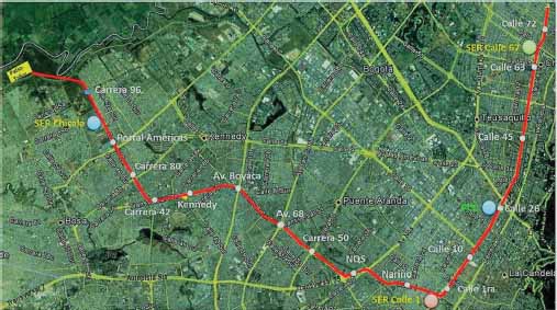
Source: Empresa Metro de Bogotá
The main parameters and electromechanical and passenger capacity characteristics of PLMB are described below (see Tables 1 to 3).
Table 1
Main characteristics of PLMB
System characteristics |
Min. |
Max. |
Demand capacity of the first phase (hour/direction passengers) |
26232 |
36000 |
Distance (km) |
20.60 |
23.60 |
Commercial speed (km/h) |
43 |
43 |
Passenger density (passengers/m2) |
6 |
8 |
Minimum comfort rate (%) |
13 |
13 |
Availability of total fleet (trains) |
|
23 |
Electric substations |
|
3 |
Source: Empresa Metro de Bogotá
Table 2
Main parameters of PLMB trains
Parameters |
6 wagons |
7 wagons |
Empty train weight (ton) |
33.33 |
39.33 |
Number of axles per car |
4 |
4 |
Approximate total weight (ton) |
200 |
230 |
Drag coefficient |
0.07 |
0.07 |
Seated passenger capacity |
44 |
36 |
Standing passenger area (m2) |
257 |
266.4 |
Maximum electric load (kW) |
34.5 |
34.5 |
Source: Empresa Metro de Bogotá
Table 3
Stations and distance between stations of PLMB
Station |
Accumulated distance [km] |
Estimated time between stations [s] |
Patio taller |
0 |
0 |
1: Carrera 96 |
1.30 |
108 |
2: Portal Américas |
2.66 |
114 |
3: Carrera 80 |
3.76 |
92 |
4: Carrera 42 |
5.01 |
104 |
5: Kennedy |
6.01 |
84 |
6: Avenida Boyacá |
7.39 |
115 |
7: Avenida 68 |
9.14 |
147 |
8: Carrera 50 |
10.05 |
76 |
9: NQS |
11.47 |
119 |
10: Nariño |
13.06 |
133 |
11: Calle Primera |
14.51 |
121 |
12: Calle Décima |
15.66 |
96 |
13: Calle 26 |
17.26 |
134 |
14: Calle 45 |
19.12 |
156 |
15: Calle 63 |
20.75 |
137 |
16: Calle 72 |
22.48 |
145 |
Total |
22.48 |
31 min, 21 s |
Source: Empresa Metro de Bogotá
2.2 Theoretical framework
The consumption of electric energy for traction, in a massive Metro-type transport system, represents between 40 per cent and 80 per cent of the total energy consumed by such a system (Domínguez et al., 2012; Yuan & Frey, 2020), that is where the importance of focusing the analysis of this energy with the aim of establishing reliable monitoring indicators in the operation and identifying potential savings, increased efficiencies and reduction in the emission of pollutants to the environment. With respect to the above, a number of authors, in recent years, have found savings potential ranging from 15 per cent (Sumpavakup et al., 2017)), to 30 percent and higher in energy (Su et al., 2016), and in the order of reduction of emissions from 15 per cent to 19 per cent (Yuan & Frei, 2020).
In the movement of a train along a route you have various forces involved: The traction force, the force of opposition to movement and the braking force. The traction force is necessary to overcome the resistance and accelerate to the train; the force of opposition to movement depends on the features of the train and the geometrıa of the way and the braking force is necessary to deceler the train until the complete stop is achieved.
In this work, the speed is considered to act as an independent variable (Jong & Chang, 2005a; Jong & Chang, 2005b), and in this sense speed profiles are generated in each section (Ahmadi et al., 2018; Sanchis & Zuriaga, 2016). The traction power is calculated with the speed profiles, the calculation of the instant force and the subsequent evaluation of the instantaneous power (F*v) in the different sections. Once this information has been obtained, and by integrating the instantaneous power in time, the result is the electric energy consumed. With the aim of determining a specific energy consumption indicator, this integration is effective taking into account the total time of the route and dividing between the total route (km)
The model for the determination of energy includes the electromechanical variables with which it can be calculated, both the energy consumed and the energy returned to the distribution system (Wang & Rakha, 2017). With the purpose of a better display, these variables are grouped in Table 4.
Table 4
Variables for energy characterization of PLMB
Variable |
Description |
Unit |
EC(t) |
Instantaneous energy consumption |
kWh |
ECre(t) |
Regenerated instantaneous energy |
kWh |
P(t) |
Instantaneous traction power |
kW |
F(t) |
Instantaneous traction force |
N |
V(t) |
Instantaneous speed |
km/h |
Wp |
Weight per axle of a wagon |
Ton |
np |
Number of axles per car |
# |
K |
Drag coefficient |
# |
L |
Distance traveled by the train per second |
m |
M |
Total train weight |
Ton |
d |
Total distance per journey |
km |
Source: Empresa Metro de Bogotá
The energy model is set as follows, according to Wang & Rakha (2017):
Equation (1) quantifies positive energy (consumed), EC(t), when the train is in traction mode; that is, when it is in motion, that is when the energy flows from the power system to the train. On the other hand, when the train is in regenerative braking mode (deceleration), (Khodaparastan et al., 2019), energy, ECre(t), flows from the train to the distribution system and is considered negative.
Where:
EC(t): Instantaneous energy consumed with moving train, [kWh]
P(t): Instantaneous traction power with moving train, [kW]
α1: Header power, [kW]
α2: Header power fraction (kW) (suggested value:0.05)
β1: Fictitious logical variable
β2: Fictitious logical variable
The terms α1 * β1 and α2 * β2 of equation (1) are related to the máximum load of the system. Constants β1 and β2 are logical values that can have values of 0 and 1. The value of 1 is applied in the largest case with β1 = 1, y β2 = 0, except when the train is standing by waiting for passengers, at which point a fraction of energy must be consider.
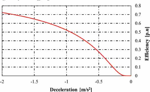
Equation (2) allows the power returned to the distribution system to be calculated and makes sense when the train is braking. In the case of efficiency, a factor to be determined by equation (3) can be calculated and checked in figure 2, in the event that the braking slow down goes up to 2 m/s2
Figure 2
Efficiency in energy regeneration based on deceleration
Where:
ECre(t): Instantaneous energy returned to the grid by regenerative braking, [kWh]
η(t): Instantaneous regenerative efficiency coefficient
Where:
α: Model calibration parameter (0.65)
ɑ(t): Instant deceleration in braking, [m/s2]
The specific energy during a journey in one direction is the sum of the two energies divided by distance, as can be seen in equation (4), with the variable d being in (km).
Where:
EC tot: Average specific energy consumed on a trip per unit distance, [kWh/(tren*km)]
d: Length travelled by the train throughout the driving cycle, [km]
The energy determined by equation (4) can be considered as a specific energy (energy intensity), as it quantifies energy per unit distance (km) and per vehicle (train).
In the case of the traction force, it may be posible to use the modified Davis equation (5), (A. R. E. Association, 1988). This equation has proven valid and has been improved by many transport engineers in order to increase their reliability.
Where:
F(t): Instantaneous traction force, [N]
Wp: Load per train axle including passengers (75kg/passanger), [ton]
np: Number of train axles
K: Drag coefficient (0.65)
V(t): Speed at instan t, [km/h]
M: Total weight of the train, including passengers, [ton]
Where:
θ: Slope of the track, [%]
Where:
L: Distance traveled by the train in one second, [m]
3. Methodology
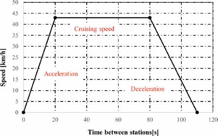
In order to estimate electricity consumption per unit distance and per vehicle, a software application was developed in matlab to generate speed profiles, as shown in figure 3. The application or program algorithm consists of the following: In the initial part, individual speed profiles are generated for each of the sections, considering an acceleration and a constant intermediate or cruising speed, which last a certain time in seconds and in the final part there is a deceleration time until reaching the complete train stop (see figure 4).
Figure 3
Flow chart of the developed application
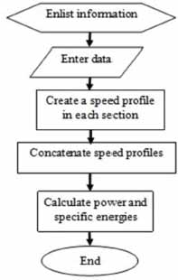
Figure 4
Example of a speed profile for a typical path in the PLMB
The technical literature (García et al., 2009; Rios & García, 2010), reports several ways to evaluate, by numerical methods, the energy consumed. One of them is to generate speed profiles (independent variable) in order to obtain energies, distances and travel times (dependent variables).
Speed profiles are generated with a constant initial acceleration of 1m/s2 up to a predefined constant or cruising speed. In the final part there is a period of deceleration varying around -1m/s2.
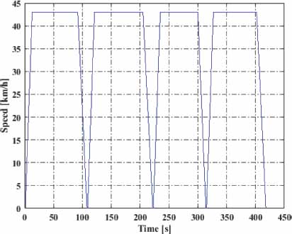
A second step in the algorithm consists of concatenating the individual profiles of the first step, to obtain the total velocity profile of the total travel, as shown in figure 5.
Figure 5
Example of a typical speed profile for a travel between four stations
In the final part, the traction force is calculated, equation (5), and the product of force and speed is made to obtain the instantaneous power, equation (8). The integration of instantaneous power, over time, determines the energy consumed, which can also be displayed as time passes.
The scenarios considered for calculating the specific energy consumed, per unit of length (km) and per vehicle, are described below.
3.1 Scenario 1: Cruising speed of 43 km/h and acceleration of 1 m/s2
A reference speed profile was initially defined with acceleration slope of 1 m/s2 and cruising speeds of 43 km/h, this for each of the 16 sections described in Table 3. Changes were made to this reference profile at cruising speed of +5 km/h and -5 km/h and of -0.2 m/s2 and +0.3 m/s2 in acceleration. The speed reference profile for all sections is seen in figure 5.
The following results were obtained:
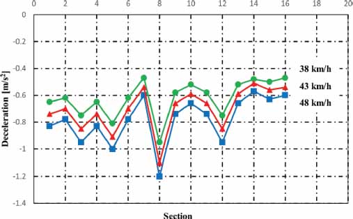
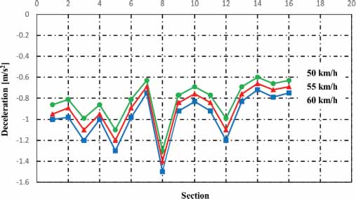
The speeds behaved as observed in figures 6 and 7. In figure 6 the average speeds in each section are observed with the reference cruising speed and with the changes in cruising speed at 38 km/h and 48 km/h. In figure 7 it is observed how the average velocities varied with changes to 0.8 m/s2 and 1.3 m/s2 in acceleration. The decelerations behaved as illustrated in figure 8. Solid lines represent average decelerations for changes in speeds at 38 km/h and 48 km/h.
Figure 6
Changes in average speeds in each section with changes in cruise speeds in scenario one
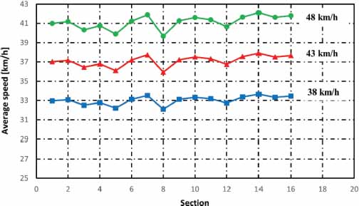
Figure 7
Changes in average speeds in each section with changes in accelerations in scenario one
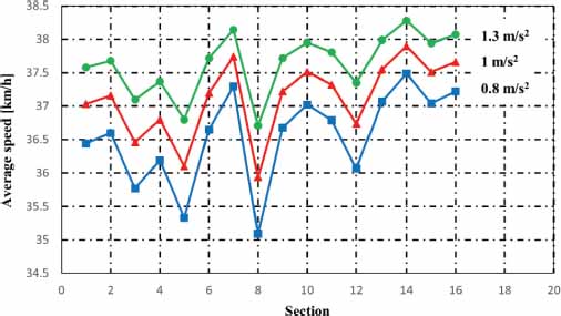
Figure 8
Changes in average decelerations in each section due to changes in cruising speed in scenario one
3.2 Scenario 2: Cruising speed of 55 km/h and acceleration of 1 m/s2
Similar to what was done in scenario 1, a speed reference profile was initially defined with acceleration slopes of 1 m/s2 and cruise speeds of 55 km/h, this for each of the 16 sections described in Table 3. On this reference profile, changes were made in cruising speed of +5 km/h and -5 km/h and of -0.2 m/s2 and +0.3 m/s2 in acceleration. The following results were obtained (see figures 9-11).
Figure 9
Changes in average speeds in each section due to changes in cruise speeds in scenario number 2
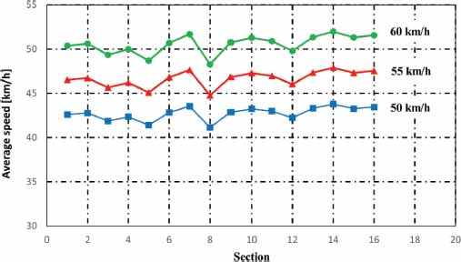
Figure 10
Changes in average speed in each section due to change in accelerations in scenario number 2
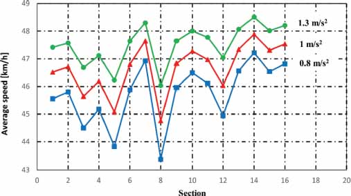
Figure 11
Changes in average decelerations in each section due to changes in cruising speed in scenario number 2
4. Results
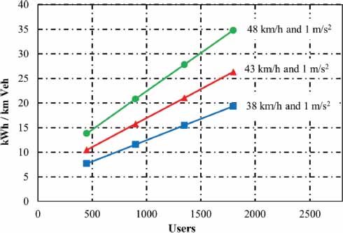
Representative results such as those shown in figures 12 and 13 were obtained for instantaneous power and energy. The following results were obtained for the indicator of specific energy consumed in the initial scenario and variations in speed above and below the reference speed of 43 km/h (See Table 5 and figure 14).
Figure 12
Power peaks at moments of acceleration, cruising speed, and deceleration
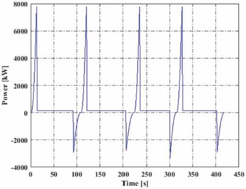
Figure 13
Integration of power and specific energy for a route
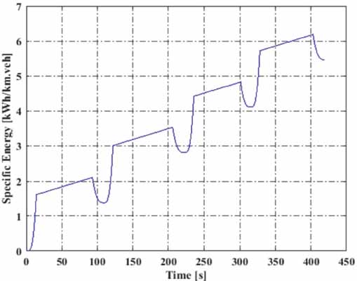
Table 5
Specific energy [kWh/km.veh] obtained in the initial scenario of speed of 43 km/h and acceleration of 1 m/s2, speed variation
Passengers |
38 km/h and 1 m/s2 |
43 km/h and 1 m/s2 |
48 km/h and 1 m/s2 |
450 |
7.68 |
10.46 |
13.82 |
900 |
11.57 |
15.75 |
20.81 |
1350 |
15.46 |
21.04 |
27.80 |
1800 |
19.34 |
26.32 |
34.79 |
Figure 14
Specific energy depending on the number of users for initial scenario and variation of the cruising speed around 43 km/h
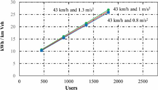
Regarding the variation of the specific energy consumption when the acceleration varies, the results shown in Table 6 and in figure 15 were obtained.
Table 6
Specific energy [kWh/km.veh] obtained in the initial scenario of speed of 43 km/h and acceleration of 1 m/s2, acceleration variation
Passengers |
43 km/h and 0.8 m/s2 |
43 km/h and 1 m/s2 |
43 km/h and 1.3 m/s2 |
450 |
10.27 |
10.46 |
10.68 |
900 |
15.46 |
15.75 |
16.08 |
1350 |
20.61 |
21.04 |
21.48 |
1800 |
25.85 |
26.32 |
26.87 |
Figure 15
Specific energy as a function of the number of users for the initial scenario and acceleration variation around 1 m/s2
Regarding the second scenario, the following results are obtained in the behavior of the specific energy when the speed and the acceleration ramp varied around the values of 55 km / h and 1 m/s2, respectively (See Tables 7 and 8 and figures 16 and 17).
Table 7
Specific energy [kWh/km.veh] obtained in the final scenario of speed of 55 km/h and acceleration of 1 m/s2, speed variation
Passengers |
50 km/h and 1 m/s2 |
55 km/h and 1 m/s2 |
60 km/h and 1 m/s2 |
450 |
13.54 |
17.28 |
21.69 |
900 |
20.38 |
26.01 |
32.66 |
1350 |
27.23 |
34.75 |
43.62 |
1800 |
34.03 |
43.5 |
54.59 |
Table 8
Specific energy [kWh/km.veh] obtained in the final scenarioof speed of 55 km/h and accele ration of m/s2, acceleration variation
Passengers |
55 km/h and 0.8 m/s2 |
55 km/h and 1 m/s2 |
55 km/h and 1.3 m/s2 |
450 |
16.94 |
17.28 |
17.7 |
900 |
25.51 |
26.01 |
26.65 |
1350 |
34.07 |
34.75 |
35.6 |
1800 |
42.64 |
43.5 |
44.54 |
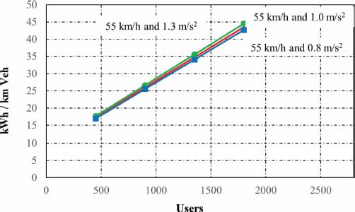
Figure 16
Specific energy depending on the number of users for the final scenario and variation of the cruising speed around 55 km/h
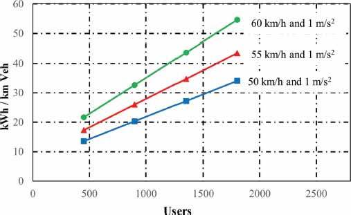
Figure 17
Specific energy depending on the number of users for the final scenario and acceleration variation around 1 m/s2
The results show a great sensitivity of the specific consumptions to changes in cruising speed (figures 14 and 16) and, on the contrary, little sensitivity or variation to changes in the acceleration ramps (figures 15 and 17).
The decelerations are greater when they have higher cruising speeds. This is evidenced in figure 8 (average deceleration of - 0.7 m/s2) vs figure 11 (average deceleration of - 0.9 m/s2). Linked to what was expressed in the previous paragraph, in scenario 1 there was an efficiency factor in regeneration of 0.39; while in scenario 2 an efficiency factor of 0.52 resulted. In other words, greater energy return is achieved when you have a higher cruising speed.
The results obtained consider a maximum acceleration ramp of 1.3 m/s2 and a maximum deceleration (in section 8, the shortest section of the entire route) of -1.5 m/s2. These maximum acceleration and deceleration values are within the typical ones reported in the technical literature, (Rios & García, 2010), for these cases of estimating energy demand.
The section 8, as it is the shortest and where the greatest deceleration occurs, could be considered to have a lower cruising speed than in the rest of the sections of the total route.
The scenario that comes closest to having a commercial speed of 43 km/h (the one specified for the system) is the one in which there is a cruising speed of 42.73 km/h and specific consumption of 13.54; 20.73; 27.23 and 34.07 kWh/km-veh for 450; 900; 1350 and 1800 passengers, respectively.
5. Conclusions
The most important conclusions of this work are the following:
It is possible to have control of the specific energy consumed, through the speed profiles in the different sections (system operation).
Having an average commercial operating speed of 43 km / h implies having to have a cruising speed of approximately 55 km / h.
Variations in accelerations have little influence on the behavior of specific energy consumptions.
The scenarios proposed allow us to identify a margin to achieve greater efficiencies in the energy return process. The average deceleration in scenario 2, higher cruising speed, turned out to be -0.9 m/s2, which could go as low as -1.5 m/s2 where there would be a coefficient in energy return of around 0.65, but the aforementioned cost to some extent sacrificing the comfort of the passengers for this greater deceleration.
It was found that higher cruising speeds would imply less travel time, but at the cost of increasing specific consumption. Consumption depends on the speed profiles and consequently on the operation of the system.
Acknowledgments
The author is grateful for the support received from the Vice-Rectory of Research and Transfer of the Universidad de La Salle, Bogotá D.C., for the development of the research project “Characterization of the energy demand for the mass transportation system (Transmilenio and Metro) in the long-term horizon 2020-2035”. Project code CUAC 19106.
References
Ahmadi, S., Dastfan, A., & Assili, M. (2018). Energy saving in metro systems: Simultaneous optimization of stationary energy storage systems and speed profiles. Journal of rail transport planning & management, 8(1), 78-90.
A. R. E. Association, Manual. Chicago: American Railway Engineering Association, 1988
Domínguez, M., Fernández-Cardador, A., Cucala, A. P., & Pecharromán, R. R. (2012). Energy savings in metropolitan railway substations through regenerative energy recovery and optimal design of ATO speed profiles. IEEE Transactions on Automation Science and Engineering, 9(3), 496-504.
Garcia, G., Rios, M. A., & Ramos, G. (2009). A power demand simulator of electric transportation systems for distribution utilities. 2009 44th International Universities Power Engineering Conference (UPEC) (pp. 1-5). IEEE.
Gao, Y., Yang, L., & Gao, Z. (2018). Energy consumption and travel time analysis for metro lines with express/local mode. Transportation Research Part D: Transport and Environment, 60, 7-27.
Gattuso, D., & Restuccia, A. (2014). A tool for railway transport cost evaluation. Procedia-Social and Behavioral Sciences, 111, 549-558.
González-Gil, A., Palacin, R., Batty, P., & Powell, J. P. (2014). A systems approach to reduce urban rail energy consumption. Energy Conversion and Management, 80, 509-524.
Jong, J. C., & Chang, E. F. (2005). Models for estimating energy consumption of electric trains. Journal of the Eastern Asia Society for Transportation Studies, 6, 278-291.
Jong, J. C., & Chang, S. (2005). Algorithms for generating train speed profiles. Journal of the eastern ASIA society for transportation studies, 6, 356-371.
Khodaparastan, M., Mohamed, A. A., & Brandauer, W. (2019). Recuperation of regenerative braking energy in electric rail transit systems. IEEE Transactions on Intelligent Transportation Systems, 20(8), 2831-2847.
Ríos, M. A., & García, G. (2010). Modelo de cálculo de demanda de potencia eléctrica en sistemas de tracción tipo metro, tren y tranvía. Revista de ingeniería, 32, 7-15.
Sanchis, I. V., & Zuriaga, P. S. (2016). An energy-efficient metro speed profiles for energy savings: application to the Valencia metro. Transportation research procedia, 18, 226-233.
Su, S., Tang, T., & Wang, Y. (2016). Evaluation of strategies to reducing traction energy consumption of metro systems using an optimal train control simulation model. Energies, 9(2), 105.
Sumpavakup, C., Ratniyomchai, T., & Kulworawanichpong, T. (2017). Optimal energy saving in DC railway system with on-board energy storage system by using peak demand cutting strategy. Journal of modern transportation, 25, 223-235.
Wang, J., & Rakha, H. A. (2017). Electric train energy consumption modeling. Applied energy, 193, 346-355.
Yuan, W., & Frey, H. C. (2020). Potential for metro rail energy savings and emissions reduction via eco-driving. Applied energy, 268, 114944.
_______________________________
1 Universidad de La Salle, Bogotá, Colombia.
ORCID: 0000-0002-8349-2551. Correo-e: lcorrea@unisalle.edu.co