CONTRIBUTION TO COMPETING SPECIES MODELING WITH DISTRIBUTED DELAY

1. Introduction

Hsu, Hubbell and Waltman have analyzed the behavior of a predator-prey system consisting of two predators' species x₁ , x₂ and a single prey specie, S (1978a, 1978b). The predator species compete purely exploitative, with no interference between rivals (no toxins are produced, for example). Both species have access to the prey and compete only by lowering the population of shared prey. For death rates it is assumed that the number dying is proportional to the number currently alive. In the absence of predation, the prey grows logistically, and the predator’s functional response obeys the Michaelis-Menten kinetic, which is also called the Holling type curve. Thus, it is assumed that if there are no significant time lags in the system, the following model may describe the situation:

Here: x_i(t) is the number of the i-th predator at time t; S(t) is the number of the prey at time t; m_i is the maximum growth rate of the i−th predator; D_i is the death rate for the i-th predator; a_i is the half-saturation constant for the i-th predator, which is the prey density at which the functional response of the predator is half maximal; γ and K are the intrinsic rate of increase and the carrying capacity for the prey population respectively. The model (1) has been extensively studied for several authors, nonetheless here a distributed delay is introduced and using the linear trick chain technique the analysis of the dynamics of the equilibria and the main properties of the model are studied. The delay system is converted by mean of linear trick chain technique in an “equivalent system” of five ordinary differential equations. The final purpose is to look for conditions where neither, one, or both species of predators survive.

2. Formulation of the model

As it was mentioned early, a modification of the predator-prey model (1) will be performed. The main consideration is that there are lags in transforming the consumed prey biomass into new biomass of the predator populations. In order to model this process of conversion of prey consumed into predators, a distributed delay is introduced in the system to describe the involved time lag. More precisely, assume in a more realistic fashion that the present level of the predators affects instantaneously the growth of the prey, but the growth of the predator is influenced by the amount of prey in the past. Thus, suppose that the predator grows up depending on the weight average time of the function of Michaelis-Menten of the prey S over the past per predator. Thus, the model takes the form of the following integro-differential system:

$$\begin{gathered} S\text{'}\left(t\right) = S\left(t\right)(1-\frac{S\left(t\right)}{K})-\frac{m_1{x}_1\left(t\right)S\left(t\right)}{a_1+S\left(t\right)}-\frac{m_2{x}_2\left(t\right)S\left(t\right)}{a_2+S\left(t\right)}, \\ {x}_1^{\text{'}} = -D_1{x}_1\left(t\right)+{\int }_{\infty }^t{a}_1{x}_1\left(\tau \right)exp(-a_1(t-\tau \left)\right)\left(\frac{m_{1}S\left(\tau \right)}{a_1+S\left(\tau \right)}\right)d\tau , \\ {x}_2^{\text{'}}\hspace{0.17em}=\hspace{0.17em}-D_2{x}_2\left(t\right) + {\int }_{-\infty }^t{\alpha }_2{x}_1\left(\tau \right)exp(-{\alpha }_2(t-\tau \left)\right)\left(\frac{m_{2}S\left(\tau \right)}{a_2+S\left(\tau \right)}\right)d\tau \end{gathered}$$

In the literature, the kernel

$K\left(u\right)=\alpha exp(-\alpha u)$ (2)

is called the weak kernel and is frequently used in biological modeling and clearly implies that the influence of the past is fading away exponentially and the number 1/α_i might be interpreted as the measure of the influence of the past respect to the predator population x_i. So, to smaller α_i, longer is the interval in the past in which the values of S are taken into account (Cushing, 1977; MacDonald, 1978). This kernel has the property that 

${\int }_{-\mathrm{\infty }}^t{\alpha }_i\exp (-{\alpha }_i(t-\tau ))d\tau ={\int }_0^{\mathrm{\infty }}{\alpha }_i\exp (-{\alpha }_{i}s)ds=1$.

The behavior of the solutions of this system of ordinary differential equations will be analyzed looking to answer under what conditions will neither, one, or both species of predators survive and give some insight from the biological point of view. The adequate space for the initial data of the problem and some related notations is as follow:

Let $B{C}_{+}^3$ denote the Banach space of the\ bounded and continuous function mapping from the interval $(-\mathrm{\infty },0]$ to ${\mathbb{R}}_{+}^3$, the 3-dimensional vectors with positive coordinates. From the general theory of integral differential equations (Burton, 2005; Miller, 1971), for any initial data $\varphi =({\varphi }_0,{\varphi }_1,{\varphi }_2)\in B_{+}^3$, there exists a unique solution $\pi (\varphi ;t):=(S(\varphi ;t),x_1(\varphi ;t),x_2(\varphi ;t))$ for all t>0 and ${\pi (\varphi ;0)|}_{(-\mathrm{\infty },0]}=\varphi$. Throughout, denote by $(S(t),x_1(t),x_2(t))$ the solution $\pi (\varphi ;t)$ with $\varphi \in B{C}_{+}^3$, when no confusion arises. By a positive solution $\pi (\varphi ;t)$ or $(S(t),x_1(t),x_2(t))$ of the previous integro-differential system, means that the solution has initial condition $\varphi \in B{C}_{+}^3$ and each component of the solution is positive for all t>0. However, the model given by the previous integro-differential system can be associated to a system ordinary differential equations in the following way: 

Introducing two new unknown functions, y_i , defined by:

$y_i(t)={\int }_{-\mathrm{\infty }}^t{\alpha }_i{x}_i(\tau )\exp (-{\alpha }_i(t-\tau ))\left(\frac{m_{i}S(\tau )}{a_i+S(\tau )}\right)d\tau$, (3)

i=1, 2 and using the form of the weak kernel (2) and the linear trick chain technique (MacDonald, 1978) gives the new system of ordinary differential equations:

$\begin{array}{rl}{S}^{\mathrm{\prime }}(t)& =S(t)(1-\frac{S(t)}{K})-\frac{m_1{x}_1(t)S(t)}{a_1+S(t)}-\frac{m_2{x}_2(t)S(t)}{a_2+S(t)}\\ x_1^{\mathrm{\prime }}(t)& =-D_1{x}_1(t)+y_1(t)\\ x_2^{\mathrm{\prime }}(t)& =-D_2{x}_2(t)+y_2(t)\\ y_1^{\mathrm{\prime }}(t)& ={\alpha }_1(\frac{m_1{x}_1(t)S(t)}{a_1+S(t)}-y_1(t))\\ y_2^{\mathrm{\prime }}(t)& ={\alpha }_2(\frac{m_2{x}_2(t)S(t)}{a_2+S(t)}-y_2(t)).\end{array}$ (4)

Thus, the integro-differential system is “equivalent” to this system of 5-dimensional ordinary differential equations. The relationship between both systems are interpreted as follows: If $(S,x_1,x_2):[0,\mathrm{\infty })\to {\mathbb{R}}_{+}^3$ is the solution of the integro-differential system corresponding to the continuous and bounded initial functions $(\tilde{S},{\tilde{x}}_1,{\tilde{x}}_2):(-\mathrm{\infty },0]\to {\mathbb{R}}_{+}^3$, then $(S,x_1,x_2,y_1,y_2):[0,\mathrm{\infty })\to {\mathbb{R}}_{+}^5$ is solution of (4) with the initial conditions $S(0)=\tilde{S}(0),x_1(0)={\tilde{x}}_{1_0},x_2(0)={\tilde{x}}_{2_0}$, with:

$y_i(0)={\int }_{-\mathrm{\infty }}^0{\alpha }_i{x}_i(\tau )\exp (-{\alpha }_i(t-\tau ))\left(\frac{m_{i}S(\tau )}{a_i+S(\tau )}\right)d\tau ,i=1,2$

Conversely, if $(S,x_1,x_2,y_1,y_2)$ is any solution of (4), defined on the entire real line and bound ed on (−∞, 0], then y_i , i=1, 2, is given by (2), so (S, x₁ , x₂ ) satisfies (3).

Most of the results of the paper are established considering the “equivalent system’’ (4).

3. Basic properties

In this section the basic properties of the model are established. In doing that, the following results are important for the proofs of some lemmas and theorems in the following. The first one is a lemma due to Barbalat and the proof may be seen in Gopalsamy (1992).

Lemma 1 (Barbălat lemma). Let a be a finite number and $\mathrm{f}:[a,\mathrm{\infty })\to \mathbb{R}$ be a differentiable function. If $\underset{t\to \mathrm{\infty }}{lim}f(t)$ exists (finite) and the derivative function g is uniformly continuous on (a, ∞), then $\underset{t\to \mathrm{\infty }}{lim}\mathrm{g}(\mathrm{t})=0$.

The next definition and the theorem are due to Markus (1956) and will be needed for the proofs of some theorem in the next section.

Definition 1 Let $A:x_i^{\mathrm{\prime }}=f_i(x,t)$ and $A_{\mathrm{\infty }}:x_i^{\mathrm{\prime }}=f_i(x)(i=1,2,\dots ,n)$ be a first order system of ordinary differential equations. The real-valued functions f_i(x, t) and f_i (x) are continuous in (x, t) for x ∈ G, where G is an open set in ${\mathbb{R}}^n$, and for t>t₀, and they satisfy a local Lipschitz condition in x. A is said to be asymptotic to $A_{\mathrm{\infty }}(A\to A_{\mathrm{\infty }})$ in G if for each compact set K ⊂ G and for each ε>0, there is a T = T(K, ε)>t₀ such that:

$|f_i(x,t)-f_i(x)|<\epsilon$ for all $i=1,2,\dots ,n$, all $x\in K$ and all $t>T\text{.}$

In relation with the previous definition, the Markus theorem follows.

Theorem 2 (Markus) Let $A\to A_{\mathrm{\infty }}$ in G and let P be an asymptotically stable critical point of A_∞. Then there is neighborhood N of P and a time T such that the omega limit set for each solution x(t) of A, which intersects N at a time later than T is equal to P.

In the following results, the well definiteness of the system (4) is described. Note that the Barbălat Lemma implies that if $(S(t),x_1(t),x_2(t),y_1(t),y_2(t))$, satisfies the system (4); then, according with the remark of Wolkowicz et al. (1997, p. 1288), each component of this solution is uniformly continuous.

The following preliminary two lemmas are basic for the well biological meaning of the integro-differential model. The first one indicates that the model possesses the property that positive initial data yield positive solutions.

Lemma 3 (Positivity) For any $\varphi \in B{C}_{+}^3$ with ${\varphi }_0>0,{\varphi }_i>0,i=1,2$, the solution $\pi (\varphi ;t)$ remains positive for all t>0.

Proof. Clearly,

$S(t)=S(0)\exp \left({\int }_0^t\{(1-\frac{S(\tau )}{K})-\frac{m_1{x}_1(\tau )}{a_1+S(\tau )}-\frac{m_2{x}_2(\tau )}{a_2+S(\tau )}\}d\tau \right)$,

and so S(t)>0 for all t>0 since S(0)>0. To show that $x_i(\varphi ;t)>0$ for all t>0 , suppose that it is not true. Let: 

$\overline{t}=\inf \{t>0:x_i(\varphi ;t)=0$ and $x_i(\theta )>0,0\le \theta <t\}<\mathrm{\infty }$,

Then $x_i(\overline{t})=0$ and $x_i^{\mathrm{\prime }}(t)\le 0$. But from the integro-differential system, the following calculation gives:

$\begin{array}{rl}{x}_i^{\mathrm{\prime }}(\overline{t})& =-D_i{x}_i(\overline{t})+{\int }_{-\mathrm{\infty }}^{\overline{t}}{\alpha }_i{x}_i(\tau )\exp (-{\alpha }_i(\overline{t}-\tau ))\left(\frac{m_{i}S(\tau )}{a_i+S(\tau )}\right)d\tau \\ & ={\int }_{-\mathrm{\infty }}^{\overline{t}}{\alpha }_i{x}_i(\tau )\exp (-{\alpha }_i(\overline{t}-\tau ))\left(\frac{m_{i}S(\tau )}{a_i+S(\tau )}\right)d\tau >0\mathrm{.}\end{array}$

This is a contradiction. Therefore, $x_i(\varphi ;t)>0$ for any positive t. This completes the proof.

Note that the previous lemma implies that the set:

$E=\{(S,x_1,x_2,y_1,y_2)\in R^5\mid S>0,x_1>0,x_2>0,y_1>0,y_2>0\}$

is invariant under the flow induced by the system (4). The following, second lemma, has to do with the property of pointwise dissipativity.

Lemma 4 (Pointwise Dissipativity) All positive solutions of model given by the integro-differential system are bounded for t>0. Moreover, system (4) is pointwise dissipative and the absorbing set B (into which every solution eventually enters and remains) is given by:

$\begin{array}{c}B=[0,K]\times [0,L\left(D_1\right)]\times [0,L\left(D_2\right)]\times \\ [0,K/p+1]\times [0,K/p+1],\end{array}$(5)

where

$L(D)=K/pD+1/D+1$ and $p=min\{1,{\alpha }_1,{\alpha }_2\}.$

Proof. Of the equation for S in (4) it is easy to see that using a similar argument, as in the proof of Lemma 3.1 in Hsu et al. (1978b), the boundedness of S(t) can be obtained. Precisely, for sufficiently small ε>0 there exists T depending only on S(0), such that S(t))<K + ε , for t>T.

Now let:

$W=S+\frac{y_1}{{\alpha }_1}+\frac{y_2}{{\alpha }_2}$

then, for t>T,

$\begin{array}{rl}{W}^{\mathrm{\prime }}& =S^{\mathrm{\prime }}+\frac{y_1^{\mathrm{\prime }}}{{\alpha }_1}+\frac{y_2^{\mathrm{\prime }}}{{\alpha }_2}\\ & =S(1-\frac{S}{K})-y_1-y_2,\\ & <K+\epsilon -S-{\alpha }_1\left(\frac{y_1}{{\alpha }_1}\right)-{\alpha }_2\left(\frac{y_2}{{\alpha }_2}\right),\\ & <K+\epsilon -p\{S-\frac{y_1}{{\alpha }_1}-\frac{y_2}{{\alpha }_2}\},\end{array}$

where p = min {1, α₁, α₂}. And so,

W’ < K − pW.

This clearly implies the uniform boundedness of y₁ and y₂. Also note that taking into account the equations for x_i in the equations (4), the boundedness of y_i (t) implies the boundedness of x_i (t). Taking into account the previous differential inequality and the equations for x_i in the system (4), the number T₁ = T₁ (ε, P₀ ) is obtained for P₀ = (S₀, x₁₀, x₂₀, y₁₀, y₂₀ ), in such a way that:

$0<S(t)<K+\epsilon ,0<x_i(t)<M_i+\frac{\epsilon }{p{D}_i},0<y_i(t)<\frac{K}{p}+1+\frac{\epsilon }{p^{\mathrm{\prime }}}$

where $M_i=K/p{D}_i+1/D_i+1$, for all t>T₁ . Thus, the pointwise dissipativity is obtained for the systems (4). This concludes the proof. 

4. Properties of the equilibrium points

The following results shall give a complete description of the global asymptotic behavior of the system (4) under the generic condition μ₁ ≠ μ₂ , where the parameter μ_i is the ratio of the i−th predator’s Michaelis-Menten (half-saturation) constant to its intrinsic rate of increase, times is death rate, i.e.,

${\mu }_i=\frac{a_i{D}_i}{m_i-D_i}.$

In this case, the equilibria of the system (4) are given by:

$\begin{array}{rl}{E}_0& =(0,0,0,0,0),\\ E_K& =(K,0,0,0,0),\\ E_1& =({\mu }_1,f_1\left({\mu }_1\right),0,D_1{f}_1\left({\mu }_1\right),0),\\ E_2& =({\mu }_2,0,f_2\left({\mu }_2\right),0,D_2{f}_2\left({\mu }_2\right)),\end{array}$

where:

The following result has to do with the inadequate predator, this result characterize the conditions under which the predators cannot survive on the prey, given the carrying capacity of the prey population, even in the absence of competition.

Lemma 5 A necessary condition for either species x_i survive is 0<μ_i < K.

Proof. If S(t) ≥ K, then S(t)<0. Therefore, taking into account the absorbing set B given in (5), suppose that S(t)<K. Now let w_i (t) = x_i (t) + y_i (t)/ α_i , i = 1, 2. Then: 

$w_i^{\mathrm{\prime }}(t)=x_i^{\mathrm{\prime }}(t)+\frac{y_i^{\mathrm{\prime }}(t)}{{\alpha }_i}=-D_i{x}_i(t)+\frac{m_i{x}_i(t)S(t)}{a_i+S(t)}.$

If m_i ≤ D_i , then the following representation is obtained:  

$w_i^{\mathrm{\prime }}(t)=x_i(t)\left(\frac{(m_i-D_i)S(t)-a_i{D}_i}{a_i+S(t)}\right).$

And if μ_i ≥ K, then the following representation is obtained:

In any case, the appropriate representation implies that the positive function w(t) is decreasing and the limit of w(t) as t goes to infinity there exists. If  $\underset{t\to \mathrm{\infty }}{lim}w(t)=w^{\ast }>0$, then by virtue of the uniform continuity of the derivatives of w(t) and the Barbălat lemma, $\underset{t\to \mathrm{\infty }}{lim}{w}^{\mathrm{\prime }}(t)=0$. Therefore, if $\underset{t\to \mathrm{\infty }}{lim sup}{x}_i(t)=d_i>0$, then there exists a sequence $\left\{t_n\right\},\underset{n\to \mathrm{\infty }}{lim}{t}_n=\mathrm{\infty }$, such that $\underset{n\to \mathrm{\infty }}{lim}{x}_i\left(t_n\right)=d_i$, and, therefore, $\underset{t\to \mathrm{\infty }}{lim}S(t)={\mu }_i$. This contradicts the fact that S(t) < K < μ_i . Thus $lim\underset{t\to \mathrm{\infty }}{sup}{x}_i(t)=0$. That concludes the proof.

The previous lemma states that, if the maximum birth rate mi is less than or equal to the death rate D_i , or if the parameter μ_i is greater or equal to the carrying capacity of the prey, then the ith predator will die out. This establishes that there is a minimum population size which can support a given predator: K must be larger than μ_i for the i−th predator survive, independent of competition. Thus, the Lemma 5 implies the following global result that describes the outcome in which both predator populations are eliminated because of an inadequate environment for either population to survive, rather than as a result of competition.

Theorem 6. If (a) m₁ ≤ D₁ or μ₁ ≥ K, and (b) m₂ ≤ D₂ or μ₂ ≥ K, then $\underset{t\to \mathrm{\infty }}{lim}S(t)=K$ and $\underset{t\to \mathrm{\infty }}{lim}{x}_i(t)=0,i=1,2$.

Proof. Clearly the hypothesis implies that $\underset{t\to \mathrm{\infty }}{lim}{x}_i(t)=0,i=1,2$, and this implies that $\underset{t\to \mathrm{\infty }}{lim}{y}_i(t)=0,i=1,2$. With this, the remainder of the proof follows applying the Markus theorem in the same way as in the proof of Theorem 3.3(i) of Hsu et al. (1978b).

In the remainder of the paper is assumed that 0<μ₁ < K.

Theorem 7. Let (a)

${\mu }_1<K<a_1+2{\mu }_{1^{\mathrm{\prime }}}$ (8)

$\frac{D_2}{m_2}<\frac{{\mu }_1}{a_2+{\mu }_1}$ (9)

${\alpha }_1<\frac{D_1{\mu }_1}{a_1}$ (10)

and (b) m₂ ≤ D₂ or μ₂ ≥ K, then the equilibrium point E₁ of the system (4) is globally asymptotically stable.

Proof. Clearly the hypothesis (b) implies that $\underset{t\to \mathrm{\infty }}{lim}{x}_2(t)=0$, and this implies that $\underset{t\to \mathrm{\infty }}{lim}{y}_2(t)=0$. In applying the Markus theorem let the system A be the system (4), and the system A_∞ be given by:

Clearly A→A_∞ in E. By other hand, the Jacobian matrix evaluated in the equilibrium point (μ₁ , f₁ (μ₁), 0, D₁ f₁ (μ₁), 0) of the system A_∞ is given by:

$\left(\begin{array}{ccccc}1-\frac{2{\mu }_1}{K}-\frac{a_1}{a_1+{\mu }_1}(1-\frac{{\mu }_1}{K})& -D_1& 0& 0& 0\\ 0& -D_1& 0& 1& 0\\ 0& 0& -D_2& 0& 1\\ \frac{{\alpha }_1{a}_1}{a_1+{\mu }_1}(1-\frac{{\mu }_1}{K})& {\alpha }_1{D}_1& 0& -{\alpha }_1& 0\\ 0& 0& \frac{{\alpha }_2{m}_2{\mu }_1}{a_2+{\mu }_1}& 0& -{\alpha }_2\end{array}\right)$

and the characteristic polynomial of this matrix is given by newline:

$p(\lambda )=p_1(\lambda )p_2(\lambda ),$

Where:

$\begin{array}{rl}A& =-\frac{{\mu }_1}{a_1+{\mu }_1}(\frac{2{\mu }_1}{K}+\frac{a_1}{K}-1),\\ B& =\frac{{\alpha }_1{a}_1}{a_1+{\mu }_1}(1-\frac{{\mu }_1}{K}),\\ C& =\frac{{\alpha }_2{m}_2{\mu }_1}{a_2+{\mu }_1}.\end{array}$

The hypothesis (9) of the theorem implies that the two roots of the polynomial p₁ have negative real part, and the hypothesis (8) implies that A<0 and B>0. Thus the Routh-Hurwitz criterion implies that all of the root of the polynomial p₂ have negative real part. Because if were, 

$({\alpha }_1+D_1-A)(-A)({\alpha }_1+D_1)\le D_{1}B,$

then:

$({\alpha }_1+D_1-A)\frac{{\mu }_1}{a_1+{\mu }_1}(\frac{2{\mu }_1+a_1}{K}-1)({\alpha }_1+D_1)\le \frac{D_1{a}_1{a}_1}{a_1+{\mu }_1}(1-\frac{{\mu }_1}{K}).$

Taking into account (8), this inequality implies that:

$(\frac{2{\mu }_1+a_1}{K}-1)\frac{{\alpha }_1+D_1}{{\alpha }_1}<\frac{a_1}{{\mu }_1}\left(\frac{{\mu }_1+a_1}{K}\right),$

after some manipulations and taking into account (10) result that K>2μ₁ + a₁ , what is contradictory with (8). Thus, the equilibrium point (μ₁ , f₁ (μ₁ ), 0, D₁f₁ (μ₁ ), 0) of the system A_∞ is asymptotically stable and by virtue of Markus lemma the conclusion of the theorem is obtained.

The following theorem guarantees the persistence of the species S, x₁ , x₂ under the necessary condition given in the previous lemma. Here the theory of uniform persistence used here is as appear in Thieme (1993).

Theorem 8. If 0<μ_i < K, i ∈ {1, 2}, then the all the populations S, x₁ , x₂ are persistent.

5. The one predator-one prey system

In order to have a comprehensive insight of the model, in this section the analysis of the one predator-one prey system is presented. In this case, the system (4) reduces to the three-dimensional system of ordinary differential given by:

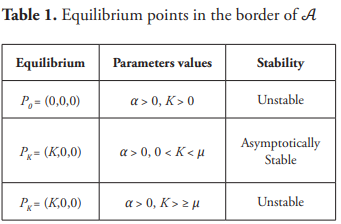
Denote by 𝒜 the open region $𝒜=\{(S,x,y)\in {\mathbb{R}}^3:S>0,x>0,y>0\}$ and define by μ, the lumping parameter given by μ = aD/m−D. It is easy to see that the only equilibrium points of system (12) in the boundary of 𝒜 are P₀ = (0, 0, 0), which is unstable, and P_K = (K, 0, 0), which is globally asymptotically for μ>K. There are not equilibrium points with positive coordinates for the previous mentioned values of the parameters. When μ = K, the equilibrium P_K loses his stability (see Table 1) and a saddle-node bifurcation arises and for μ<K appears the only equilibrium, P_* in the positive orthant, which is given by:

$P_{*}=(\mu ,f(\mu ),Df(\mu ))$, where $f(S)=1/m(1-S/K)(a+S).$

Letting u = (S, x, y)T, v = (S, x, z)T, and H=diag [1, 1, −1]. The transformation v = Hu takes the system (12) into a competitive and irreducible system in the sense as appears in Smith (2008). Note that system (12) may be written as:

$\begin{array}{rl}& S^{\mathrm{\prime }}=h(S)(f(S)-x)\\ & y^{\mathrm{\prime }}=\alpha (h(S)x-y),\end{array}$

where h(S) = mS/a+S. With these notations, the Jacobian matrix of system (13) evaluated at the equilibrium point P_* takes the form:

$\begin{array}{rl}A& =\left(\begin{array}{ccc}h(\mu )f^{\mathrm{\prime }}(\mu )& -h(\mu )& 0\\ 0& -D& 1\\ \alpha h^{\mathrm{\prime }}(\mu )f(\mu )& \alpha h(\mu )& -\alpha \end{array}\right)\\ & =\left(\begin{array}{ccc}\left(\frac{D}{mK}\right)(K-a-2\mu )& -D& 0\\ 0& -D& 1\\ \left(\frac{aD\alpha }{mK\mu }\right)(K-\mu )& \alpha D& -\alpha \end{array}\right)\end{array}$

and the characteristic polynomial of the matrix A is given by:

$p(\lambda )={\lambda }^3+b^2{\lambda }^2+b_1\lambda +b_0$

where,

$\begin{array}{rl}{b}_2& =\alpha +D+\left(\frac{D}{mK}\right)(a+2\mu -K),\\ b_1& =\left(\frac{D(\alpha +D)}{mK}\right)(a+2\mu -K),\\ b_0& =\left(\frac{a{D}^2\alpha }{mK\mu }\right)(K-\mu ).\end{array}$

To see the sign of the real part of the roots of the polynomial p(λ), the Routh-Hurwitz criterion will be used. Clearly, if K>a + 2μ, then the equilibrium point P_* is unstable since the coefficient b₁ is negative. Therefore, the stability of the equilibrium point P_* requires filling the condition:

$\mu <K<a+2\mu$ (14)

The Routh-Hurwitz criterion implies that negative the real part of the roots of p(λ) occurs if and only if the following inequality hold:

$(\alpha +D-G)(\alpha +D)G>\alpha L,$ (15)

where G = (D/mK) (a + 2μ − K) and L = aD2 /mKμ (K − μ). From this inequality the following polynomial is obtained:

$q(\alpha ,K)=G(\alpha +D{)}^2+(G^2-L)(\alpha +D)+DL.$

Where the parameter K is emphasized as an argument of the polynomial q in order to explain better his sign as α varies respect to K. The inequality (15) holds, if and only if, q(α, K)>0. The sign of the polynomial q(α, K) depends on the coefficient of the term α + D. By other hand, the function q has a minimum respect to α at α_* + D = − 1/2 r(K)/G, given by:

$q({\alpha }_{\ast },K)=\frac{1}{2G}((r(K){)}^2+L)-(\frac{Gr(K)}{2}+DL).$ (16)

When this minimum is positive, then clearly q(α, K)>0 and the equilibrium point is stable for all K>μ. Now, putting:

$r(K)=G^2-L,$ (17)

and note that r(μ) is positive, and r(a + 2μ) is negative, which implies that there exists a unique value of K between μ and a + 2μ, say K_* , such that r(K_*) = 0. Thus, for K in the interval (μ, K_* ], r(K) ≥ 0, and therefore the coefficient (17) of the term α+D of the polynomial q(α, K) is positive, which implies that q(α, K)>0, for all positive α, and in this case the equilibrium point P_* is (locally) asymptotically stable. When K ∈ (K_* , a + 2μ), the sign of r(K) reversed and in this case the coefficient of the term α+D of the polynomial q(α, K) (17) is negative. In this case, q(α, K) has two zeros α₁ + D, α₂ + D, such that q(α, K) ≤ 0 for α ∈ (α₁ + D, α₂ + D) and the equilibrium point P_* is unstable. Note that all of this situation occurs when the minimum of q(α, K) is negative, and clearly:

$\frac{{\alpha }_1+{\alpha }_2}{2}={\alpha }_{\ast }.$ (18)

All of the previous calculations are summarized in the following theorem. The proof of the Hopf bifurcation isnvolve several calculations and the procedure is similar to the used in in Cavani & Farkas (1994).

Theorem 9. A necessary condition for the existence of the equilibrium of positive coordinates P_* of the system (12) is μ<K. Moreover: (i) If μ<K<a + 2μ, then there exists a unique number K_* between μ and a + 2μ such that if K belongs to the interval (μ, K_* ), the equilibrium P_* is (locally) asymptotically stable for all positive α. When K = K * , the equilibrium P_* is a center (stable). For K>K_* the equilibrium point P_* , lost its stability and for K in the interval (K_* , a + 2μ) there are two values of α, α₁ and α₂ such that for α ∈ (α₁ + D, α₂ + D), q(α, K) in (16) is negative and therefore the equilibrium P_* is unstable. If K = K_* and α = α₁ + D, a transcritical Hopf bifurcation takes place. Finally, for K ≥ a + 2μ the coefficient b₁ of the characteristic polynomial p(λ) of the matrix A is negative and therefore the equilibrium point P_* is unstable.

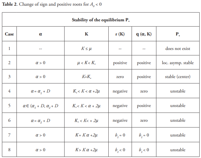
Note from (17) that for K<K_* very near to the value K_* the term r(K) is positive and the equilibrium point P_* goes from to be stable to unstable as K passes through K_* and α through α₁ + D . This can be interpreted as the system (13) exhibits the paradox of the enrichment; however, the delay may act as a mechanism to regain the stability. In fact, when 1/α increases and passes through 1/α₁ +D, the equilibrium point P_* is again stable. The Table 2 that follows may be useful in order to get in mind the stability of the equilibrium P_* .

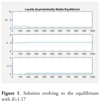
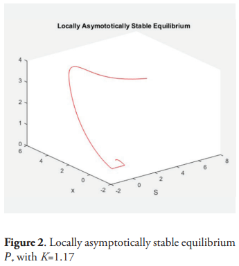
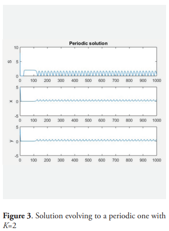
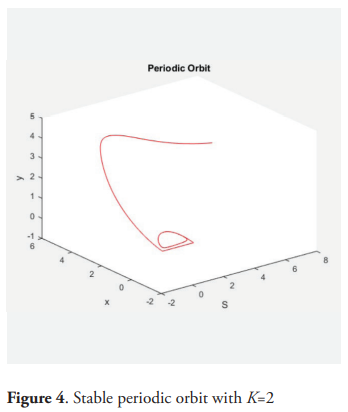
Example. For the following values of the parameters: m = 2, a = 0.5, D = 1, give μ = 0.5, a + 2μ = 13.5, K_* = 1.18. and picking K = 1.17, then for α = 0.9 the equilibrium point P_* is (locally) asymptotically stable. For K = 2 and α = 0.9 there is a stable periodic orbit.

6. Conclusions 

This paper is an analysis of the behavior of a model of two predators competing exploitatively for a shared prey species. The prey grows logistically in absence of predation and the predators consume prey according to a saturating functional response, but the growth of the predator is influenced by the amount of prey in the past. It is supposed that the predator grows up depending on the weight average time of the function of Michaelis-Menten of S over the past per predator. The system is equivalent to a dissipative system of five ordinary differential equation, by using the so-called trick of the linear chain. The analysis of this equivalent system establishes that the species survive if and only if K>μ_i, where K is the carrying capacity of the prey specie and μ_i is the ratio of the i−th predator according with the Michaelis-Menten response. The case when there exists only one predator is analyzed with detail. In this case the equilibrium point of positive coordinates is unstable for all K>a + 2μ. Theorem 9 characterizes the general situation and the occurrence of the Hopf bifurcation. The table 2 describes all of the situations analyzed and the figures 1, 2, 3 and 4 give examples of the dynamic.